Maximizing OCT in the Diagnosis and Management of Glaucoma
This technology has become an integral part of glaucoma care, and optometrists must understand how to accurately use it.
By Danica Marrelli, OD
Release Date: May 15, 2020
Expiration Date: May 15, 2023
Estimated Time to Complete Activity: 2 hours
Jointly provided by Postgraduate Institute for Medicine (PIM) and Review Education Group
Educational Objectives: After completing this activity, the participant should be better able to:
- Discuss OCT findings and common concerns with the technology.
- Use OCT to confirm a diagnosis of glaucoma.
- Follow glaucoma patients with serial macular and RNFL scans.
- Avoid common concerns related to OCT technology.
Target Audience: This activity is intended for optometrists engaged in the care of patients with glaucoma.
Accreditation Statement: In support of improving patient care, this activity has been planned and implemented by the Postgraduate Institute for Medicine and Review Education Group. Postgraduate Institute for Medicine is jointly accredited by the Accreditation Council for Continuing Medical Education, the Accreditation Council for Pharmacy Education, and the American Nurses Credentialing Center, to provide continuing education for the healthcare team. Postgraduate Institute for Medicine is accredited by COPE to provide continuing education to optometrists.
Faculty/Editorial Board: Danica Marrelli, OD, University of Houston College of Optometry.
Credit Statement: This course is COPE approved for 2 hours of CE credit. Course ID is 67937-GL. Check with your local state licensing board to see if this counts toward your CE requirement for relicensure.
Disclosure Statements:
Dr. Marrelli has received consulting fees from Aerie, Allergan, Bausch & Lomb, Carl Zeiss Meditec and fees for non-CE/CME services from Aerie, Bausch & Lomb, Carl Zeiss Meditec.
Managers and Editorial Staff: The PIM planners and managers have nothing to disclose. The Review Education Group planners, managers and editorial staff have nothing to disclose.
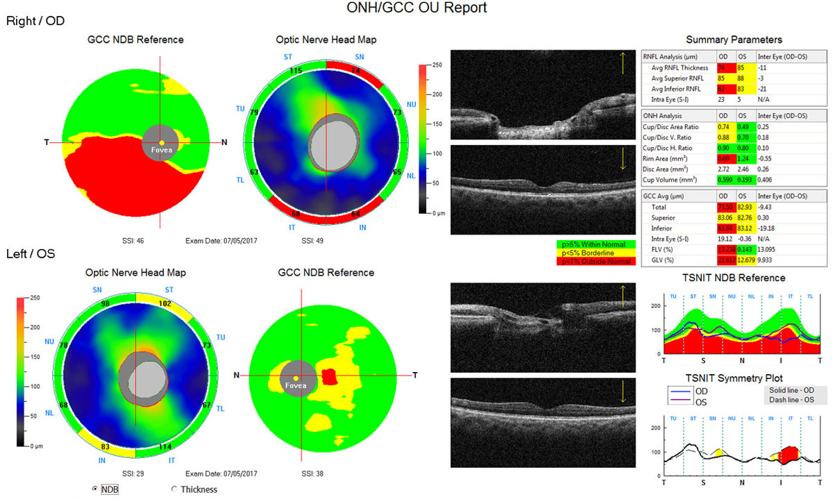 |
| Fig. 1. This Optovue OCT scan shows thinning of the inferior RNFL (absence of “warmer” greens/yellows, and more “cool” blue inferior to the disc) and the inferior ganglion cell complex (presence of red areas below the horizontal) in the right eye. On the lower right portion of the printout, the RNFL is plotted against the normative/reference database, where the inferior RNFL of the right eye dips well into the abnormal “red” range. Below that, the symmetry plot color-codes areas of significant asymmetry between the right and left eye. Click image to enlarge. |
Glaucoma can be defined as a chronic, progressive loss of retinal ganglion cells (RGCs) that results in characteristic structural—optic nerve head (ONH) and retinal nerve fiber layer (RNFL)—damage and corresponding functional (visual field) loss. Historically, clinicians relied on clinical assessment (ophthalmoscopy and fundus photography) of the ONH and RNFL to identify the structural changes. However, detecting glaucomatous changes in optic nerves can be a difficult task and one in which there is poor interobserver agreement.1-3
Over the past two decades, objective imaging with optical coherence tomography (OCT) has become increasingly important in the diagnosis of glaucoma. The diagnostic accuracy of all commercially available spectral-domain OCT instruments is similar and improves with increasing severity of the disease.4-8 This activity discusses the technology and provides a practical approach to analyzing the printouts.
OCT Scan Protocols
Although differences in scan protocols exist between manufacturers, there are three anatomic regions that can be imaged that provide important information: the ONH, RNFL and macula.
Optic nerve head and retinal nerve fiber layer. The ONH/RNFL scan is presently the most popular scan protocol used in glaucoma diagnostics. The scan provides information about the ONH, including disc size/area, rim area and cup-to-disc ratio. The neuroretinal rim thickness profile is also displayed. The RNFL data typically includes a thickness map, deviation map, RNFL thickness profile and average/global, quadrant and sector/clock hour thicknesses.
After ensuring that the patient demographic information is correct, the first step when interpreting an ONH/RNFL scan is to ensure that it is high quality without obvious artifacts or acquisition errors. The optic disc should be well-centered within the fixed measuring circle, well illuminated and relatively free of motion artifacts (indicated by discontinuous blood vessel path or irregularly shaped optic nerve). The signal-to-noise ratio (i.e., signal strength) should be high. Since the RNFL thickness is derived from within the defined measuring circle, based on the specific machine used, it is critical that there are no black areas (indicating missing data) within the circle that will affect the average, quadrant or sector thickness measurement. After ensuring good scan quality, the clinician can move on to choosing the scan analysis and interpreting the findings.
A color-coded RNFL thickness map allows a rapid “first glimpse.” In this thickness map, warm colors (reds and oranges) represent areas of thick RNFL and cooler blues represent thinner areas. The normal thickness map will show a symmetrical hourglass or butterfly shape of thick RNFL superiorly and inferiorly correlating with the anatomical location of RNFL bundles.
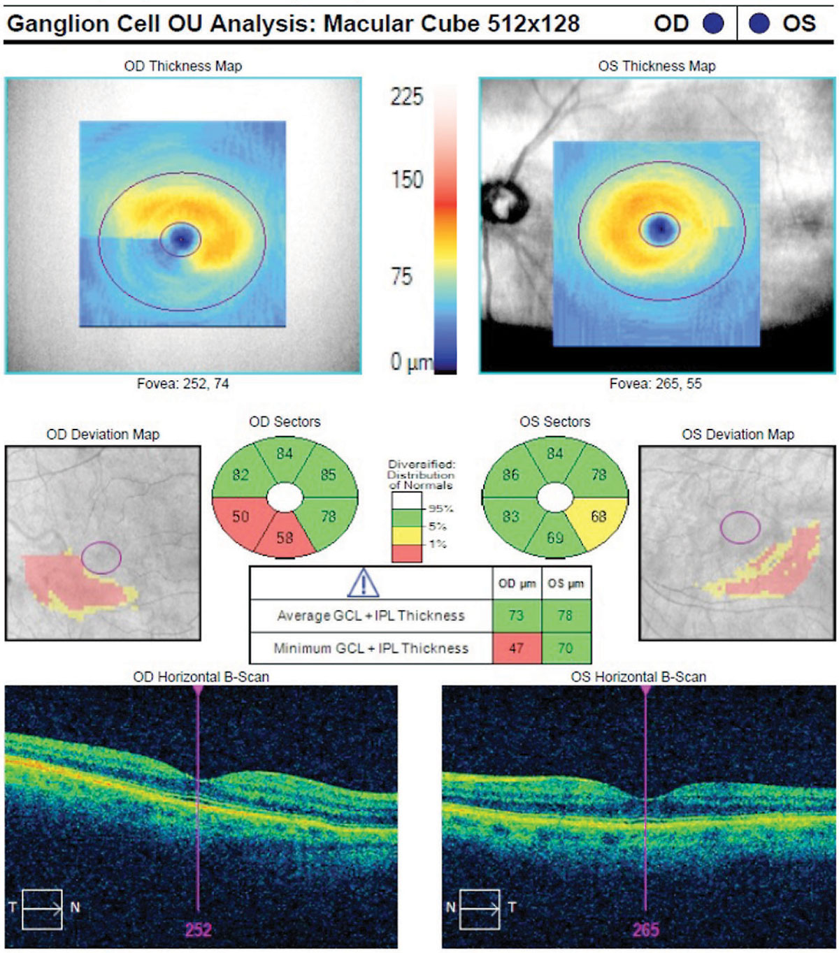 |
| Fig. 2. This macular ganglion cell analysis scan shows the characteristic wedge-shaped loss in the inferior temporal macular vulnerability zone. Note the squeegee sign more pronounced in the right eye. Click image to enlarge. |
Looking for symmetry is extremely important in all OCT scans in glaucoma, as asymmetry is a hallmark of early disease (Figure 1). A first look at symmetry can take place with the thickness map, looking to see if the thickness appears symmetric between superior and inferior thickness within each eye and between the right and left eye. Diffuse and focal (slit/wedge) RNFL loss may be identifiable as cooler colors on the thickness map. The deviation map will identify areas that are outside normal limits based on the instrument’s reference database. Yellow pixels are considered “borderline” and represent the thinnest 5% of the reference database (only 5% of normals fall within this range) and red pixels are considered “abnormal” and represent the thinnest 1% of the normative database.
While examining the deviation map, the clinician should look for loss in areas consistent with glaucoma (superior/superotemporal and inferior/inferotemporal). RNFL thickness measurements obtained from the measuring circle are presented on the report as global/average, quadrant and sector/clock hour measurements, with the color-coded indicators of green, yellow and red for the 95%, 5% and 1% thickness percentiles of the reference database, respectively. These color codes are helpful in identifying potential problem areas, but the clinician should avoid diagnosing patients based strictly on the color maps.
Arguably the most important areas to examine on the ONH/RNFL scan are the profile curves. These provide a visual representation of the optic nerve neuroretinal rim and RNFL thickness in a “TSNIT” pattern: starting with the temporal thickness, moving to superior, nasal, inferior and back to temporal for both rim and RNFL thickness.
Another profile map gaining popularity is the NSTIN curve, which splits the RNFL in the nasal hemifield rather than temporal to allow for better viewing of the susceptible temporal area of loss common in the macula. The neuroretinal rim profile may identify diffuse or focal rim thinning, which should correlate with the clinical examination of the optic nerve. A normal neuroretinal rim profile will usually demonstrate thicker rims inferiorly and superiorly, correlating with the “ISNT Rule” of clinical ONH assessment.
The TSNIT curve of the RNFL should show peaks superiorly and inferiorly; often the superior RNFL will show a “double hump” related to blood vessel positioning. The neuroretinal rim and RNFL profile curves are overlaid on the reference database color coding. Dips into the yellow/red zones should arouse suspicion but, again, are not diagnostic of disease. When the profile curves of the right and left eye are superimposed, it is easy to identify areas of asymmetry. Depending on the instrument, other parameters such as disc size, rim area and cup-to-disc ratio may also be presented on the ONH/RNFL scan.
Macula. The newest area of interest in imaging for glaucoma diagnosis is the macula. It’s long been known that glaucomatous damage can occur there.9 However, these subtle changes cannot be seen on clinical exam. OCT has revolutionized our ability to evaluate and quantify macular thickness. There are several reasons to consider the macula in early glaucoma.
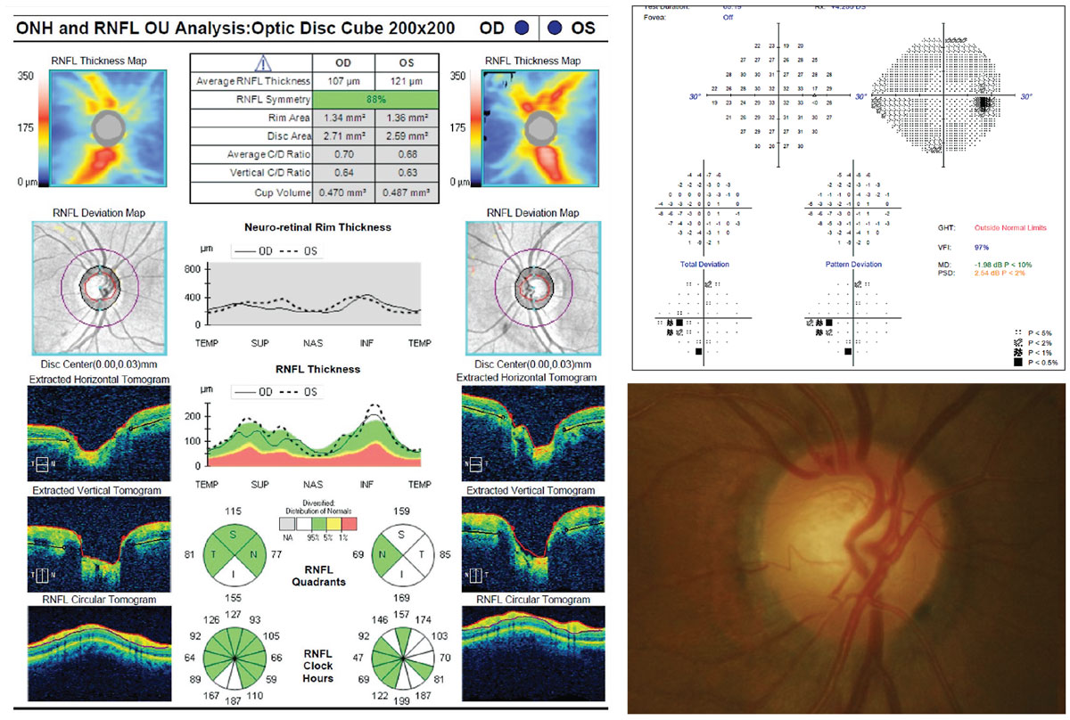 |
| Fig. 3. This OCT scan represents a case of green disease. The RNFL deviation map appears clear, and the ONH/RNFL summary table and RNFL quadrant and clock hour analyses are all in the green. However, on careful evaluation of both the thickness maps and the RNFL TSNIT profile, it is clear that the superior RNFL is thinner than the inferior RNFL in the right eye. This asymmetry is characteristic of early glaucoma. This example also shows why correlating the OCT findings with the clinical exam is important. On exam, the patient had a slightly thin superior neuroretinal rim in the right eye, and a small optic disc hemorrhage on the superior rim. In addition, there was a corresponding inferior nasal step visual field defect. Intraocular pressure, while in the statistically normal range, was consistently 3mm Hg to 4mmHg higher in the right eye on each visit. Click image to enlarge. |
First, the macula is the region of the retina with the highest density of RGCs, the cells impacted by glaucomatous damage. The central 16° of the retina contains approximately 50% of the RGCs.10,11 Since glaucoma is a disease of RGCs, it makes sense to look in the area of highest ganglion cell population.
Second, unlike the optic nerve and peripapillary region, where a wide variation of normal exists, the macula is more uniform among patients, and the measurements can be more repeatable. In healthy individuals, there is greater superior/inferior symmetry of the macular thickness than that of the peripapillary RNFL, and in all individuals there is less impact of large blood vessels in the macular area compared with the RNFL. In terms of diagnostic capability, research shows the macular scans that use inner retina segmentation are comparable with RNFL scans.4
Much of our understanding of the macula in glaucoma comes from the work of Donald Hood, PhD. In an extensive body of work, his team of researchers has identified the most likely area of early ganglion cell loss in the macula. This area, termed the “macular vulnerability zone,” is located just inferotemporal to the fovea and is commonly the site of early glaucomatous damage.12
Macular scan protocols for glaucoma vary in terms of what is measured (the entire retinal thickness or only a segment of the inner retina), and if segmented, which layers are included. For example, the ganglion cell complex is a segmentation of the inner retina including the ganglion cell, inner plexiform and RNFL.
The ganglion cell analysis is a segmentation that includes only the ganglion cell and inner plexiform layers (GCIPL). Scans are centered on the fovea and the thickness may be reported as sector, average and minimum. In addition, the Heidelberg Spectralis instrument performs a detailed macular thickness symmetry analysis, comparing superior to inferior within an eye as well as thickness of right eye compared with the left eye.
A macula of normal thickness has a uniform oval appearance on the thickness map. A hallmark of glaucomatous damage to the macula appears as a distinct loss temporal to the fovea along the horizontal raphe, which is easily visible on the thickness map (Figure 2). This appearance has been given several nicknames, including the “squeegee sign” (because it looks as if part of the inferior macula has been wiped away) and the “nautilus” (for its similarity to a nautilus shell).
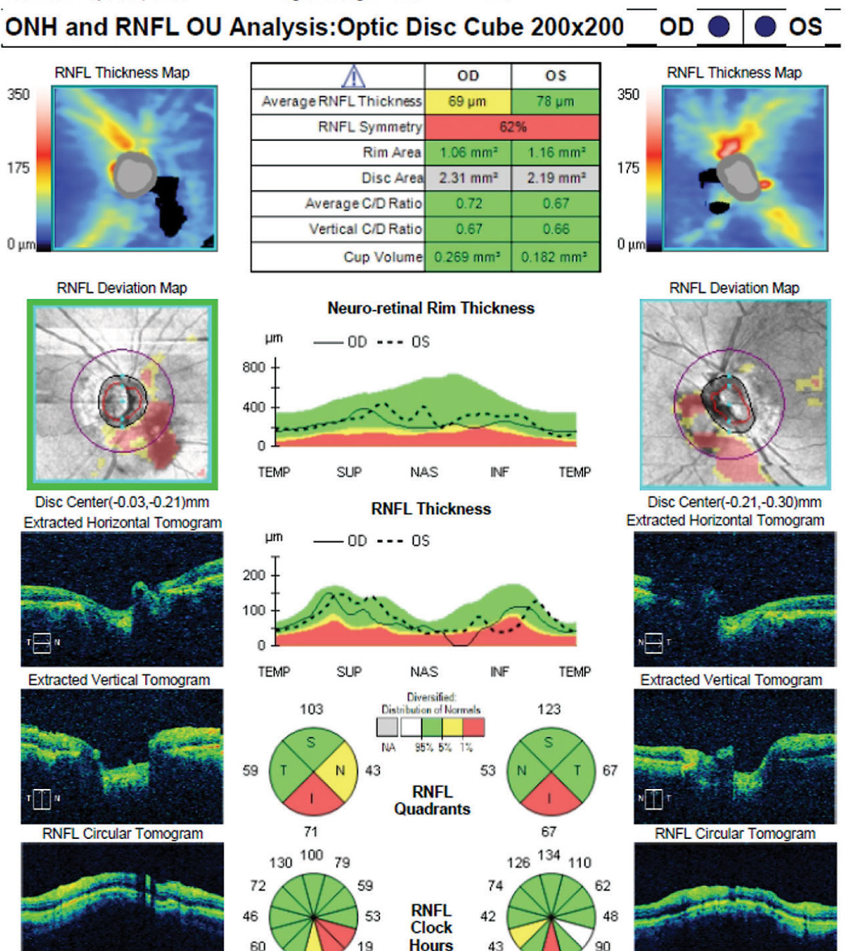 |
| Fig. 4. In this scan, large vitreous floaters in both eyes obscured the signal and created black areas within the measuring circle, which influenced the RNFL thickness measurements. In addition, note the irregular shape of the optic nerve OS and the discontinuous blood vessels in the deviation map of the left eye, indicating a motion artifact. Click image to enlarge. |
Macular OCT scans have limited usefulness for glaucoma diagnostics in the presence of macular disease, particularly disease that involves the inner retina. Macular edema, epiretinal membranes and age-related macular degeneration all alter the thickness of the macula and the capability of the instrument to segment the various layers. In patients with concomitant macular disease, macular scans are unlikely to be helpful in the diagnosis of glaucoma.13
Our new understanding of the importance of macular damage in early glaucoma has necessitated a change in the way we think about perimetry. Conventional visual field testing using either the 24-2 or 30-2 testing strategy may miss or underestimate the functional loss of damage to the macular area. In these test patterns, stimulus spacing of six degrees does not allow for adequate sampling in the central area with the highest population of retinal ganglion cells.14-16
By using a test strategy that includes closer stimulus spacing (for example, the two-degree spacing of the 10-2 or the central points of new 24-2C test pattern), clinicians may be able to improve their ability to detect early functional loss related to the macular damage.9
Currently, it’s not entirely clear which patients may benefit from central 10° visual field testing. In cases with glaucomatous ganglion cell loss and a normal 24-2 test, the 10° testing may be beneficial.
The Pitfalls of OCT
While OCT technology has greatly improved our ability to evaluate the structural loss in glaucoma, it is imperative that clinicians understand its potential pitfalls.
Normative database. Each instrument compares scans against a reference database of patients without ocular or systemic disease. OCT instruments provide color-coded reports to alert the clinician that a numeric value falls within or outside of the normal range relative to the reference database. Typically, green represents the top 95% thickness of the reference base and is considered normal; white represents the very thickest of the normative database and may be normal or may represent abnormally thick RNFL (such as in optic disc swelling). Yellow is considered borderline, representing the thinnest 5% of the database, and red is considered abnormal, representing the thinnest 1% of the database.
These databases are limited in size and with regard to age, ethnicity, optic disc size and refractive error. Because of the limitations of the databases, some patients without disease will fall outside of the normal range. These patients’ reports will flag them as red on the printouts.
The term “red disease” describes these patients who, despite being healthy, are flagged as abnormal on the OCT printout.17 Red disease is a false positive, and without carefully evaluating the individual components of the scan and considering the scan in the context of the entire clinical picture, these patients may be incorrectly diagnosed and unnecessarily treated for glaucoma.
Non-glaucomatous Conditions For example, in AION, clinicians would expect optic disc pallor rather than the cupping seen in glaucoma. In some optic neuropathies, including toxic/nutritional and ethambutol-induced optic neuropathy and dominant optic atrophy, temporal RNFL thinning is a feature that can help differentiate the condition from glaucoma.32,33 Retinal conditions that affect one hemifield, such as retinal detachment and branch retinal artery and vein occlusions, may also produce superior/inferior asymmetric RNFL loss that mimics that of glaucoma. Again, the clinical examination should provide information to arrive at the appropriate diagnosis, although in the case of a chronic/resolved branch retinal artery occlusion, the clinical examination of the retina may appear quite normal. In this situation, an important OCT feature is atrophy and thinning of the inner retinal layers in the area of the occlusion, which may be seen on raster/line scans through the retina.34 |
In a study of 104 normal eyes, researchers found a false positive glaucoma classification in 40.4% of eyes based on ganglion cell analysis and in 30.8% of eyes based on RNFL maps.18 They found that false positive classification was associated with increased axial length and small optic disc size, a finding supported by other investigators.19,20 They recommend clinicians carefully evaluate the location and pattern of loss in eyes with abnormal OCT maps.
Likewise, some patients with glaucoma will have scans in which all numeric values fall within the normal range of the reference database. These false negatives, termed “green disease,” may result in underdiagnosis and a delay in treatment of patients with glaucoma.21
In a busy practice, it is easy to become overly reliant on the red/yellow/green color scheme to make a diagnosis of glaucoma. There are two key steps in avoiding red and green disease misdiagnosis.
The first is to correlate the OCT findings with other clinical exam findings (Figure 3). The OCT should augment, not replace, the doctor’s clinical examination of the optic nerve and RNFL.
The second is to examine the scan for findings consistent with glaucoma: superior/inferior loss of neuroretinal rim and RNFL; sharply demarcated inferotemporal or superotemporal ganglion cell loss in the macula; and asymmetry between the right and left eyes (often seen easily on the superimposed TSNIT curves).
Artifacts. These occur in a surprising number of RNFL and macular scans. Researchers found that 15.2% to 36.1% of RNFL and macular scans in one glaucoma clinic population had artifacts, most of which were evident on the clinical printout.22 Other authors report up to 90% of scans have artifacts, although not all artifacts will have clinically significant implications, and many are not reproducible on repeat scans.13,23-25 Recognizing artifacts is critical to accurately interpreting the data.
Artifacts can be classified into three categories: those related to acquisition/technician errors, ocular pathology and software (segmentation) errors.
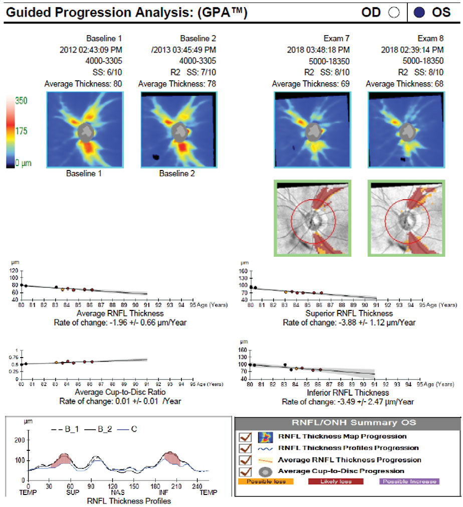 |
| Fig. 5. Here, event analysis shows significant change from baseline indicated by yellow and red pixels in the deviation from baseline maps (green boxes) and on the TSNIT profile. There is also visible thinning over time on the thickness maps, as the average RNFL thickness drops from 80µm to 68µm. Trend analysis shows a significant rate of change in average, superior and inferior RNFL as well as an increase in the cup-to-disc ratio. Click image to enlarge. |
Technician errors may include truncation of the image, such that not all of the image is included in the acquisition window. These errors will result in areas with near zero thickness and are easily recognized. Remember that the RNFL and GCIPL floor is approximately 45µm, representing residual glial and vascular tissue. Improper circle placement on ONH/RNFL scans is another potential acquisition error, although many instruments now have algorithms that make this less likely.
Poor signal-to-noise ratio may be due to media problems such as cataract or dry eye.26 Pupil dilation and slight movement in the x- (right/left) and y- (superior/inferior) axes may allow the scan to work around central lens opacities. The use of an artificial tear immediately prior to acquisition may minimize the impact of ocular surface dryness. Train technicians to recognize these acquisition errors and to re-scan the patient to minimize their impact on interpretation.
Any ocular pathology that alters retinal thickness may cause an artifact in a glaucoma scan protocol (Figure 4). The most common ocular pathology to cause artifacts is epiretinal membrane. Vitreoretinal interface disorders and epiretinal membrane may alter the thickness of the retina, as well as diminish the instrument’s ability to properly segment the retinal layers. High myopia causes thinning of both the RNFL and ganglion cell layers, and highly myopic eyes may also have anatomic features (including ONH tilting, peripapillary atrophy, myopic staphyloma and temporal RNFL bundle shifting) that may impact structural assessment of the ONH and RNFL.13,23
Software-related artifacts are primarily related to improper segmentation of the retinal layers. Poor signal strength related to media opacities and ocular surface disease may hinder the proper segmentation and impact thickness measurements. Vitreous floaters may focally obscure the signal from the retina, resulting in the inability to segment portions of the scan. Asking the patient to move their eye just prior to acquiring the scan may reposition the floaters long enough to work around them. In addition, high myopia is a frequent cause of improper segmentation in RNFL and macular scans.
Some instruments allow for manual re-segmentation of improperly segmented scans. Recognition and, when possible, correction of segmentation errors is important for accurate interpretation of the scan.
Artifacts may be a source of red/green disease. Poor signal strength, acquisition errors, vitreous floaters and myopic RNFL thinning may result in a false positive (red or abnormal) findings. Vitreoretinal interface disorders, myelinated nerve fiber layer and optic disc edema may result in false negative (green) findings.
| Pearls & Pitfalls of OCT Interpretation | |
Pearls:
| Pitfalls:
|
Detecting Progression
Once a patient is diagnosed with glaucoma, or a glaucoma suspect has entered into a surveillance program for observation, the focus shifts from diagnosis to detecting progression. Structural progression may be detected as progressive RNFL thinning, ONH changes such as rim thinning, progressive inner macular thinning or a combination of all three. Two main strategies exist for detecting progression using OCT: event analysis and trend analysis.
In event analysis, progression is detected when the difference between a baseline and follow-up scan exceeds a predetermined amount, usually the instrument’s test-retest variability (Figure 5). Clinicians can think of this as a snapshot in time that answers the question, “Has the patient changed significantly from baseline?” Typically, the first time a scan shows progression, it will be flagged in yellow (“possible progression”), and if the same progression is verified on a subsequent exam, the progressing area will be flagged in red (“likely progression”).
In general, more emphasis is placed on event analysis when there are fewer follow-up examinations (Figure 6). Interestingly, the most common location for progressive RNFL thinning is outside of the standard 3.4mm measuring circle. This means that some RNFL thinning may be identified on the thickness change map but not on the serial analysis of the circumpapillary RNFL thickness measurements, necessitating analysis of the entire scan, not one particular parameter.27
Trend analysis provides regression analysis between a given parameter and time. Progression is defined as a significant negative slope of the parameter in question. This slope can be considered a surrogate for the rate of change of the disease. Average and hemifield RNFL thickness measurements, cup-to-disc ratio and inner macula thickness can all be analyzed this way. Color indicators note when rates of change reach statistical significance.
When analyzing an OCT for progression, clinicians should remember that current OCT progression analysis software does not account for the normal age-related thinning of RNFL and macula. A number of studies have investigated the rate of RNFL loss in both healthy and glaucomatous eyes. One study showed that the average RNFL in healthy subjects changed at a rate of -0.48µm/year, while the RNFL of glaucoma patients changed at a rate of -0.98µm/year.28 In this study, rates of RNFL change were more rapid than that of GCIPL change. Other researchers found that accounting for age-related loss significantly impacted the percentage of patients determined to be progressing.29 Research also shows that failure to consider age-related thinning resulted in significant false positive identification of progression.30
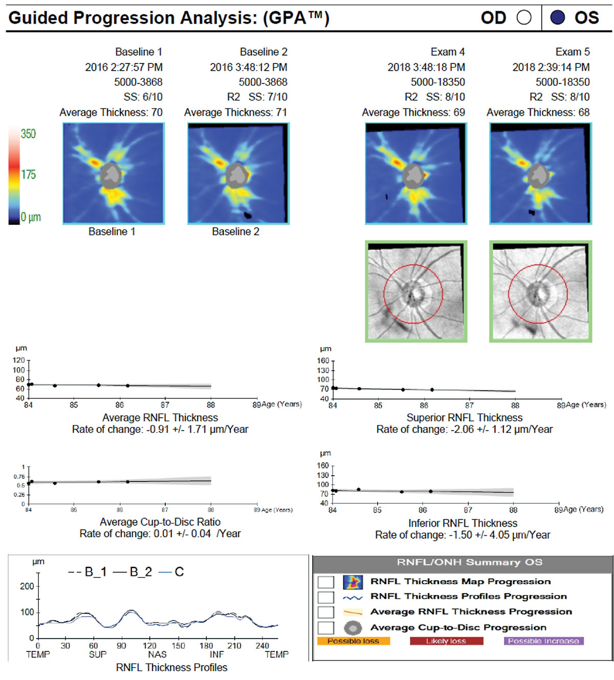 |
| Fig. 6. The patient in Figure 5 was lost to follow-up and was not using his glaucoma medication. When he returned for care and drop therapy was re-initiated, the baseline was reset to the first two scans following his return. The results of both event and trend analyses show that he has remained relatively stable since re-initiation of therapy. Click image to enlarge. |
In addition to age-related loss, clinicians should consider the severity of the disease. The ability of OCT to detect RNFL thinning diminishes in more advanced disease, as the RNFL measurement reaches the floor effect. Inner macular thickness, however, is often more useful for progression detection in advanced disease, as more GCIPL is likely to remain above the measurement floor for a longer period of time.29
Finally, a positive correlation exists between signal-to-noise ratio and RNFL thickness, so consider the scan quality (particularly compared with baseline) when evaluating for possible progression.
Always confirm suspected progression with repeat testing. If progression is confirmed, clinicians still have several decisions to make. First, they must decide if any statistically significant change is clinically relevant. Life expectancy and disease severity may play a role. For example, a change (or rate of change) that is alarming in a younger patient with moderate disease might be less clinically meaningful in an older patient with mild disease.
In addition to the clinical relevance of a change, the optometrist should consider whether the change is consistent with glaucoma or if there is another explanation for the change, such as cataract formation. If the change is deemed glaucomatous, other considerations include the time it took to reach that change (rate of progression), what the intraocular pressure and medication adherence was during that time period and the impact of the next intervention (additional medication, laser or incisional surgery) on the patient’s quality of life.
OCT helps detect progression, but clinicians must carefully decide what to do with all the information at their disposal.31 Finally, if a therapeutic change is warranted due to progression, the clinician must reset the baseline of both structural and functional testing to follow for progression from the point of the therapeutic intervention.
OCT has revolutionized our ability to qualitatively and quantitatively assess the optic nerve, RNFL and macular changes that occur in glaucoma. It has become indispensable in our decision-making in glaucoma and other diseases. By understanding the technology, its abilities and potential pitfalls, optometrists can be well prepared to use this tool in the diagnosis and management of glaucoma.
Dr. Marrelli is a clinical professor and assistant dean of Clinical Education of the Ocular Diagnostic and Medical Eye Service at the University of Houston College of Optometry.
1. Breusegem C, Fieuws S, Stalmans I, et al. Agreement and accuracy of non-expert ophthalmologists in assessing glaucomatous changes in serial stereo optic disc photographs. Ophthalmology. 2011;118(4):742-6. 2. Azuara-Blanco A, Katz LJ, Spaeth GL, et al. Clinical agreement among glaucoma experts in the detection of glaucomatous changes of the optic disk using simultaneous stereoscopic photographs. Am J Ophthalmol. 2003;136(5):949-50. 3. Varma R, Steinmann WC, Scott IU. Expert agreement in evaluating the optic disc for glaucoma. Ophthalmology. 1992;99(2):215-21. 4. Kansal V, Armstrong JJ, Pintwala R, et al. Optical coherence tomography for glaucoma diagnosis: An evidence based meta-analysis. PLoS One. 2018;13(1):e0190621. 5. Mwanza JC, Durbin MK, Budenz DL, et al. Glaucoma Diagnostic accuracy of ganglion cell-inner plexiform layer thickness: comparison with nerve fiber layer and optic nerve head. Ophthalmology. 2012;119(6):1151-8. 6. Fallon M, Valero O, Pazos, M, et al. Diagnostic accuracy of imaging devices in glaucoma: a meta-analysis. Surv Ophthalmol. 2017;62(4):446-61. 7. Oddone F, Lucenteforte E, Michelessi M, et al. Macular versus retinal nerve fiber layer parameters for diagnosing manifest glaucoma: a systematic review of diagnostic accuracy studies. Ophthalmology. 2016;123(5):939-49. 8. Sullivan-Mee M, Ruegg CC, Pensyl D, et al. Diagnostic precision of retinal nerve fiber layer and macular thickness asymmetry parameters for identifying early primary open-angle glaucoma. Am J Ophthalmol. 2013;156(3):567-77. 9. Hood DC, Raza AS, de Moraes CG, et al. Glaucomatous damage of the macula. Prog Retin Eye Res. 2013;32:1-21. 10. Curcio CA, Allen KA. Topography of ganglion cells in human retina. J Comp Neurol. 1990;300(1):5-25. 11. De Moraes CG, Song C, Liebmann JM, et al. Defining 10-2 visual field progression. Ophthalmology. 2014;121(3):741-9. 12. Hood DC. Improving our understanding, and detection, of glaucomatous damage: An approach based upon optical coherence tomography (OCT). Prog Retin Eye Res. 2017;57:46-75. 13. Wong JJ, Chen TC, Shen LQ, et al. Macular imaging for glaucoma using spectral-domain optical coherence tomography: a review. Semin Ophthalmol. 2012;27(5-6):160-6. 14. Hood DC, Raza AS, de Moraes CG, et al. The nature of macular damage in glaucoma as revealed by averaging optical coherence tomography data. Trans Vis Sci Tech. 2012;1(1):3. 15. Traynis I, De Moraes CG, Raza AS, et al. Prevalence and nature of early glaucomatous defects in the central 10° of the visual field. JAMA Ophthalmol. 2014;132(3):291-7. 16. Grillo LM, Wang DL, Ramachandran R, et al. The 24-2 visual field test misses central macular damage confirmed by the 10-2 visual field test and optical coherence tomography. Trans Vis Sci Tech. 2016;5(2):15. 17. Chong GT, Lee RK. Glaucoma versus red disease: imaging and glaucoma diagnosis. Curr Opin Ophthalmol. 2012;23(2):79-88. 18. Kim KE, Jeoung JW, Park KH, et al. Diagnostic classification of macular ganglion cell and retinal nerve fiber layer analysis differentiation of false positives from glaucoma. Ophthalmology. 2015;122(3):502-10. 19. Seo S, Lee CE, Jeong JH, et al. Ganglion cell-inner plexiform layer and retinal nerve fiber layer thickness according to myopia and optic disc area: a quantitative and three-dimensional analysis. BMC Ophthalmol. 2017;17(1):22. 20. Yamashita T, Sakamoto T, Yoshihara N, et al. Correlations between retinal nerve fiber layer thickness and axial length, peripapillary retinal tilt, optic disc size, and retinal artery position in healthy eyes. J Glaucoma. 2017;26(1):34-40. 21. Sayed MS, Margolis M, Lee RK. Green disease in optical coherence tomography diagnosis of glaucoma. Curr Opin Ophthlamol. 2017;28(2):139-53. 22. Asrani S, Essaid L, Alder BD, et al. Artifacts in spectral-domain optical coherence tomography measurements in glaucoma. JAMA Ophthalmol. 2014;132(4):396-402. 23. Awadalla MS, Fitzgerald J, Andrew NH, et al. Prevalence and type of artefact with spectral domain optical coherence tomography macular ganglion cell imaging in glaucoma surveillance. PLoS One. 2018;13(12):e0206684. 24. Hwang YH, Kim MK, Kim DW. Segmentation errors in macular ganglion cell analysis as determined by optical coherence tomography. Ophthalmology. 2016;123(5):950-8. 25. Liu Y, Simavli H, Que CJ, et al. Patient characteristics associated with artifacts in Spectralis optical coherence tomography imaging of the retinal nerve fiber layer in glaucoma. Am J Ophthalmol. 2015;159(3):565-76. 26. Hardin JS, Taibbi G, Nelson SC, et al. Factors affecting Cirrus-HD OCT optic disc scan quality: a review with case examples. J Ophthalmol. 2015;746150. 27. Leung CK. Diagnosing glaucoma progression with optical coherence tomography. Curr Opin Ophthalmol. 2014;25(2):104-11. 28. Hammel N, Belghith A, Weinreb RN, et al. Comparing the rates of retinal nerve fiber layer and ganglion cell-inner plexiform layer loss in healthy eyes and in glaucoma eyes. Am J Ophthalmol. 2017;178:38-50. 29. Leung CKS, Ye C, Weinreb RN, et al. Impact of age-related change of retinal nerve fiber layer and macular thickness on evaluation of glaucoma progression. Ophthalmology. 2013;120(12):2485-92. 30. Wu Z, Saunders LJ, Zangwill LM, et al. Impact of normal aging and progression definitions on the specificity of detecting retinal nerve fiber layer thinning. Am J Ophthalmol. 2017;181:106-13. 31. Weinreb RN, Garway-Heath DF, Leung C, et al, eds. World Glaucoma Association Consensus Series 8: Progression of Glaucoma. Kugler Publications; 2011. 32. Rosdahl JA, Asrani S. Glaucoma masqueraders: diagnosis by spectral domain optical coherence tomography. Saudi J Ophthalmol. 2012;26(4):433-40. 33. Pasol J. Neuro-ophthalmic disease and optical coherence tomography: glaucoma look-alikes. Curr Opin Ophthalmol. 2011;22(2):124-32. 34. Rodrigues IA. Acute and chronic spectral domain optical coherence tomography features of branch retinal artery occlusion. BMJ Case Rep. 2013;2013:bcr2013009007. |